Fastest Matrix NMS in the West (Part 2): Going Down to CUDA

This is the second part of a series discussing and optimizing the Matrix NMS algorithm introduced in SOLOv2. In the first part, we implemented the algorithm using regular PyTorch operations. It was simple and readable, but much slower than torchvision.ops.nms.

To improve it, I wrote a custom CUDA implementation. Simply translating every PyTorch operation to a CUDA kernel would not help much. We also need to reduce the number of intermediate tensors, kernel launches, and global memory accesses.

The implementation discussed here is available at fast-matrix-nms.

What do we need to compute?

Let the boxes be sorted by confidence score, highest first. We form a triangular IoU matrix $O \in \mathcal{R}^{N \times N}$, where each entry contains the IoU between a box and one of its higher-scoring father boxes.

For the Gaussian version used by the CUDA implementation, the candidate decay factor contributed by father box $i$ to box $j$ is

$$d_{ij} = \exp\left(\frac{O_{max,i}^2 - O_{ij}^2}{\sigma}\right),$$

where $O_{max,i}$ is the maximum overlap between box $i$ and its own father boxes. The final score is

$$s'_j = s_j \min_i d_{ij}.$$

The naive implementation expresses this almost literally:

1. Build the IoU matrix.
2. Reduce it once to obtain $O_{max}$.
3. Broadcast $O_{max}$ back to matrix shape.
4. Build an entire decay matrix.
5. Reduce it again to obtain one decay factor per box.
6. Multiply the scores and apply a threshold.

These operations can run in parallel, but they also create many intermediate tensors. Each PyTorch operation can launch a new kernel, read its inputs from global memory, and write its output back. Repeatedly moving an $N \times N$ matrix is expensive.

The CUDA version keeps the same algorithm, but turns the above list into three steps:

1. Compute tiled IoUs and the first partial max reduction together.
2. Reduce the partial maximums to one value per box.
3. Compute candidate decayed scores and mark boxes for removal directly.

The second step may take more than one kernel launch, depending on the number of boxes.

PyTorch extension

The public interface is a small C++/CUDA extension¹. The extension still sorts the scores and reorders the boxes through the PyTorch C++ API; the custom kernels take over afterward.

at::Tensor scores_sorted, order;
std::tie(scores_sorted, order) =
    scores.sort(/*stable=*/true, /*dim=*/0, /*descending=*/true);

auto boxes_sorted = boxes.index_select(0, order).contiguous();

The sort stays outside the custom kernels because PyTorch already provides an efficient implementation. The reordered boxes are made contiguous so that the IoU kernel can load them efficiently.

The extension also means the whole operation looks roughly like a regular PyTorch op:

keep = fast_matrix_nms(boxes, scores, threshold)

No Python loop is involved in the actual suppression.

Optimization 1: tile the IoU matrix

The implementation divides the matrix into $16 \times 16$ tiles. A CUDA block has the same shape:

const int dim = 16;
dim3 const block_size(dim, dim);

Each block loads two groups of 16 boxes into shared memory². Those 32 boxes produce up to 256 pairwise IoUs, so each coordinate loaded from global memory is reused many times.

__shared__ T boxes[dim * 2 * 4];
__shared__ T iou[dim * dim];

// Load two groups of boxes into shared memory first.
// One thread then computes one pairwise IoU.
iou[tid] = boxIoU(
    boxes + threadIdx.y * 4,
    boxes + (dim + threadIdx.x) * 4
);

Because boxes are already sorted by score, only one triangular half of the matrix is useful. Blocks above that triangle return immediately, and threads on a diagonal tile skip pairs that do not represent a father-child relationship. The skipped entries are filled with zero, which does not affect the later max operation.

The PyTorch implementation in Part 1 uses the upper triangle. The CUDA implementation uses the lower triangle because the roles of the rows and columns are reversed. Both represent the same father-box relationships.

This removes close to half of the IoU calculations. The full matrix is still allocated because the pairwise IoUs are needed by the last stage.

The fixed tile size also means that the number of boxes must be a multiple of 16. This avoids boundary checks in the kernels. The caller can trim the candidates after the initial confidence filtering.

Optimization 2: fuse IoU with the first reduction

Once a tile of IoUs is in shared memory, immediately writing it out and launching another kernel to read the same values for max() would be wasteful. Instead, the IoU kernel also reduces every row of the tile.

if (threadIdx.x < dim / 2)
    warpReduce(iou + threadIdx.y * dim, threadIdx.x);

if (threadIdx.x == 0)
    partial_max[row * partial_stride + blockIdx.x] =
        iou[threadIdx.y * dim];

There are 16 threads along each row, and they belong to the same warp. We can find the maximum using four fixed steps in shared memory:

sdata[lid] = max(sdata[lid], sdata[lid + 8]);
sdata[lid] = max(sdata[lid], sdata[lid + 4]);
sdata[lid] = max(sdata[lid], sdata[lid + 2]);
sdata[lid] = max(sdata[lid], sdata[lid + 1]);

The full $N \times N$ IoU matrix is written once because we need it later. The reduction output is much smaller: one partial maximum per row per 16-column tile. The first reduction happens while the values are still in shared memory.

The IoU calculation, triangular masking, and the first part of max() now share one kernel and one shared-memory tile.

Optimization 3: finish the max reduction

After the first kernel, each row has about $N/16$ partial maximums. The next stage repeatedly reduces groups of 16 in place:

$$\left\lceil\frac{N}{16}\right\rceil \rightarrow \left\lceil\frac{N}{16^2}\right\rceil \rightarrow \dots \rightarrow 1.$$

Each pass uses the same row-wise max operation. The output overwrites the beginning of the buffer, so we do not allocate a new tensor at every level. For the box counts in the benchmark, this only takes a few launches.

There is also a triangular shortcut in these kernels. A box only has father boxes before it in score order, so reduction blocks that cannot contain a valid value return without touching memory.

Optimization 4: never construct the decay matrix

The next optimization removes the decay matrix and its reduction.

The naive implementation computes all candidate decay factors, finds the minimum for each box, multiplies its score, and finally asks whether the result is below a threshold $t$:

$$s_j \min_i d_{ij} < t.$$

Since $s_j$ is non-negative, this is equivalent to

$$\exists i: s_j d_{ij} < t.$$

We do not need the minimum value if the only output we care about is whether the final score survives. Each thread computes one candidate decayed score. If it falls below the threshold, that thread marks the box for removal.

const T candidate = exp(
    (iou_max[col] * iou_max[col] - iou[row][col] * iou[row][col]) * 2
) * score[row];

if (candidate < threshold)
    drop[row] = true;

The multiplication by 2 corresponds to the hard-coded $\sigma=0.5$ used by this implementation. The source also contains the linear formula, selected as a compile-time option.

This final kernel combines broadcasting, the Gaussian function, score multiplication, and thresholding. It avoids allocating an $N \times N$ decay tensor and avoids a separate minimum reduction.

The iou_max and score values for each tile are first stored in shared memory. They can then be reused by all threads in that tile.

Multiple threads may write true to the same drop flag, but no thread changes it back to false.

Removed work

Compared with the naive PyTorch implementation, the custom path removes or shrinks several expensive pieces:

• Box coordinates are loaded into shared memory per tile instead of fetched independently for every pair.
• Roughly half of the pairwise IoUs are never calculated.
• The first IoU max-reduction is included in the IoU kernel.
• Later max-reduction passes reuse one small buffer.
• The decay matrix is never allocated or written.
• The minimum decay reduction disappears entirely.
• Broadcasting, score decay, and thresholding become one final pass.

The $O(N^2)$ work and storage for the IoU matrix remain. The implementation is faster because it reduces the work around that matrix and reuses values in shared memory.

Benchmark

The repository benchmark used random bounding boxes and torch.utils.benchmark on an NVIDIA RTX 2060 with a Ryzen 7 4800H CPU.

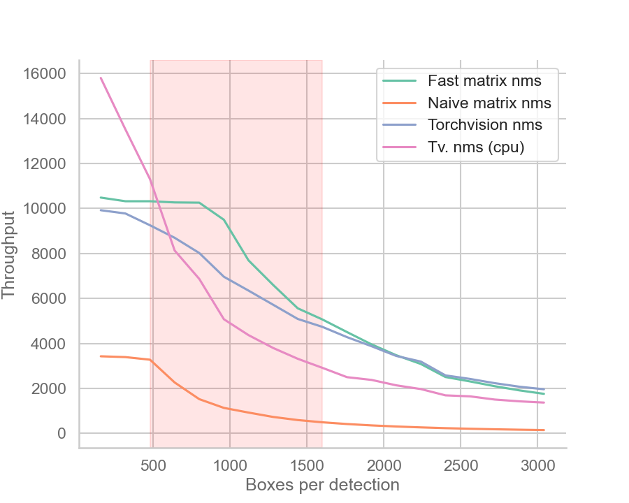
The custom implementation was around 3× faster than the naive version at the small end of the test and more than 10× faster as the number of boxes grew. In roughly the 500–1500 box range, it also had higher throughput than both the CPU and CUDA torchvision.ops.nms runs on that machine.

The curves converge as the workload grows. With more boxes, the GPU reaches its parallel computation limit and the cost of the IoU matrix and memory accesses becomes more significant.

This is only a microbenchmark. Matrix NMS and Hard NMS use different suppression rules, and the script uses different thresholds for them. Hard NMS runtime also depends on the input boxes. The result only shows that the custom implementation is much faster than the naive Matrix NMS implementation and can be competitive with torchvision.ops.nms for some input sizes.

Conclusion

The naive version also ran on the GPU, but it used many separate PyTorch operations. The custom version is faster mainly because it reuses data in shared memory, combines related operations into the same kernel, and avoids constructing the decay matrix.

The last optimization is especially useful. Since we only need to know which boxes pass the threshold, we do not need to calculate and store the final decay factor. This removes an entire matrix and one reduction from the implementation.

Footnotes

1. See the PyTorch documentation for C++ and CUDA extensions. ↩

2. See NVIDIA’s CUDA Programming Guide for an introduction to threads, blocks, warps, and shared memory. ↩